Examples
This page provides illustrative examples demonstrating how to use Mica.jl for changepoint detection across a range of domains. Before you go through this page, we recommend you to first familirize yoursef with the algorithm in Tutorial: Understanding Mica's Changepoint Detection Algorithm page.
Example 1: Toy SIR Model with Synthetic Data
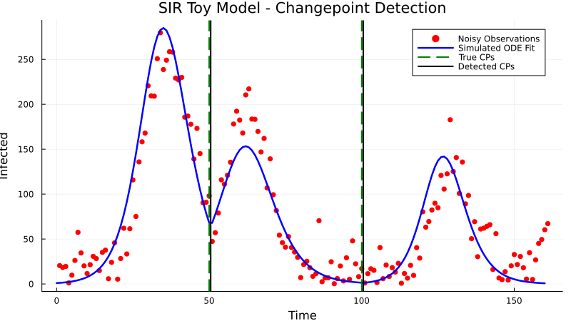
This example demonstrates detecting changepoints in a simple SIR (Susceptible-Infectious-Recovered) epidemic model with synthetic data. The infection rate (β) changes at specific points in time.
using Evolutionary, DifferentialEquations, LabelledArrays, Plots, Statistics, Random

# Define the SIR model dynamics
function sirmodel!(du, u, p, t)
    S, I, R = u
    β, γ = p
    du[1] = -β * S * I
    du[2] = β * S * I - γ * I
    du[3] = γ * I
end

# Generate synthetic data with changepoints
function generate_toy_dataset(beta_values, change_points, γ, u0, tspan, noise_level, noise)
    data_CP = []
    all_times = []
    for i in 1:length(change_points)+1
        tspan_segment = i == 1 ? (0.0, change_points[i]) :
                        i == length(change_points)+1 ? (change_points[i-1]+1.0, tspan[2]) :
                        (change_points[i-1]+1.0, change_points[i])
        params = @LArray [beta_values[i], γ] (:β, :γ)
        prob = ODEProblem(sirmodel!, u0, tspan_segment, params)
        sol = solve(prob, saveat = 1.0)
        data_CP = vcat(data_CP, sol[2,:] + noise_level * noise(length(sol.t)))
        all_times = vcat(all_times, sol.t)
        u0 = sol.u[end]
    end
    return all_times, abs.(data_CP)
end

# Setup parameters
β_values = [0.00009, 0.00014, 0.00025, 0.0005]
change_points_true = [50, 100, 150]
γ = 0.7
u0 = [9999.0, 1.0, 0.0]
tspan = (0.0, 160.0)
Random.seed!(1234)
noise_level = 20
noise = randn

# Generate data and reshape
_, data = generate_toy_dataset(β_values, change_points_true, γ, u0, tspan, noise_level, noise)
data_M = reshape(Float64.(data), 1, :)
plot(data_M[1, :])

# Redefine model with named parameters
function sirmodel!(du, u, p, t)
    S, I, R = u
    β, γ = p.β , p.γ
    du[1] = -β * S * I
    du[2] = β * S * I - γ * I
    du[3] = γ * I
end

# Wrapper for Mica
function example_ode_model(params, tspan::Tuple{Float64, Float64}, u0::Vector{Float64})
    prob = ODEProblem(sirmodel!, u0, tspan, params)
    sol = solve(prob, Tsit5(), saveat=1.0, abstol = 1.0e-6, reltol = 1.0e-6)
    return sol[:, :]
end

# Loss function for fitting
function loss_function(observed, simulated)
    simulated = simulated[2:2, :]
    return sqrt(sum(abs2, (observed .- simulated).^2))
end

# Prepare model and settings
initial_chromosome = [0.69, 0.0002]
parnames = (:γ, :β)
bounds = ([0.1, 0.0], [0.9, 0.1])
u0 = [9999.0, 1.0, 0.0]
model_spec = ODEModelSpec(example_ode_model, initial_chromosome, u0, tspan)
model_manager = ModelManager(model_spec)
n_global, n_segment_specific = 1, 1
min_length, step = 10, 10
ga = GA(populationSize=150, selection=uniformranking(20),
        crossover=MILX(0.01, 0.17, 0.5), mutationRate=0.3,
        crossoverRate=0.6, mutation=gaussian(0.0001))
my_penalty(p, n) = 10.0 * p * log(n)
n = length(data_M)

# Detect changepoints
detected_cp, params = detect_changepoints(
    objective_function,
    n, n_global, n_segment_specific,
    model_manager,
    loss_function,
    data_M,
    initial_chromosome, parnames, bounds, ga,
    min_length, step, my_penalty
)
Example 2: COVID-19 Intervention Detection in Germany
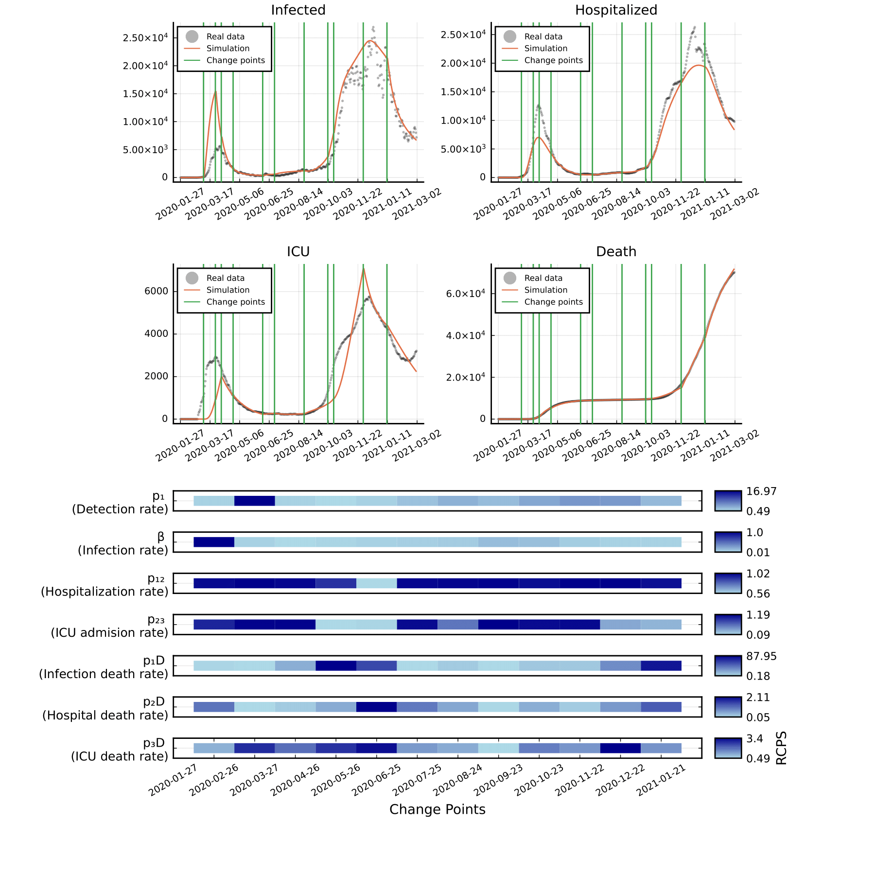
This example demonstrates Mica's application for analyzing the effects of governmental interventions during the COVID-19 pandemic in Germany.
The model includes:
11 state variables including: susceptible, multiple stages of infection, deaths, recovered, and vaccination.
8 segment-specific parameters re-estimated for each detected segment.
8 global parameters re-optimized after each new changepoint is detected.
The objective function uses five observational signals:
Infected
Hospitalized
ICU admissions
Deaths
Vaccination
A logarithmic transformation is applied to each signal before loss computation to normalize the magnitude of variation. The optimization and detection pipeline uses a tailored genetic algorithm and domain-informed parameter bounds.
After executing the Mica changepoint detection routine, most of the inferred changepoints corresponded to known intervention periods, such as lockdowns or vaccination policy shifts. This result affirms Mica’s practical utility for epidemiological modeling and policy evaluation.
📌 Note: Due to the use of real datasets, this example requires importing and pre-processing COVID-19 time series data from official RKI sources (CSV files).
We begin by defining an ODE-based epidemiological model for simulating the spread of COVID-19. To account for seasonal variation in transmission rates, a seasonality function is incorporated directly into the infection dynamics. The model is then wrapped with a solver function using the DifferentialEquations.jl package, which allows for accurate and efficient numerical integration.
using Evolutionary
using DifferentialEquations
using LabelledArrays
using Plots
using Statistics
using Random
using CSV
using DataFrames

# seasonal factor
function fδ(t::Number, δ::Number, t₀::Number=0.0)
    return 1 + δ*cos(2*π*((t - t₀)/365))
end

function log_transform(data, threshold=1e-3)
    return [val > threshold ? log(val) : val for val in data]
end

# ODE model
function CovModel!(du,u,p,t)
    (ᴺS, ᴺE₀, ᴺE₁, ᴺI₀, ᴺI₁, ᴺI₂, ᴺI₃,ᴺR, D, Cases, V) = u[1:11]
    N = ᴺS + ᴺE₀ + ᴺE₁ + ᴺI₀ + ᴺI₁ + ᴺI₂ + ᴺI₃ + ᴺR + D

    ᴺε₀  = p.ᴺε₀
    ᴺε₁  = p.ᴺε₁
    ᴺγ₀  = p.ᴺγ₀
    ᴺγ₁  = p.ᴺγ₁
    ᴺγ₂  = p.ᴺγ₂
    ᴺγ₃  = p.ᴺγ₃
    ᴺp₁  = p.ᴺp₁
    ᴺp₁₂ = p.ᴺp₁₂
    ᴺp₂₃ = p.ᴺp₂₃
    ᴺp₁D = p.ᴺp₁D
    ᴺp₂D = p.ᴺp₂D
    ᴺp₃D = p.ᴺp₃D
    δ    = p.δ
    δₜ = fδ(t,δ)
    ᴺβ   = p.ᴺβ
    ω    = p.ω
    ν = t < 330 ? 0 : p.ν

    ᴺβᴺSI = ᴺβ * δₜ * ᴺS * (ᴺE₁ + ᴺI₀ + ᴺI₁)
    du[1]  = - (ᴺβᴺSI)/N + ω * ᴺR - ν * ᴺS
    du[2]  =  (ᴺβᴺSI/N) - (ᴺε₀ * ᴺE₀)
    du[3]  =  (ᴺε₀ * ᴺE₀) - (ᴺε₁ * ᴺE₁)
    du[4]  =  ((1 - ᴺp₁) * ᴺε₁ * ᴺE₁) - (ᴺγ₀ * ᴺI₀)
    du[5]  =  (ᴺp₁ * ᴺε₁ * ᴺE₁) - (ᴺγ₁ * ᴺI₁)
    du[6]  =  (ᴺp₁₂ * ᴺγ₁ * ᴺI₁) - (ᴺγ₂ * ᴺI₂)
    du[7]  =  (ᴺp₂₃ * ᴺγ₂ * ᴺI₂) - (ᴺγ₃ * ᴺI₃)
    du[8]  =  ᴺγ₀ * ᴺI₀ + (1 - ᴺp₁₂ - ᴺp₁D) * ᴺγ₁ * ᴺI₁ + (1 - ᴺp₂₃ - ᴺp₂D) * ᴺγ₂ * ᴺI₂ +(1 - ᴺp₃D)* ᴺγ₃ * ᴺI₃ - ω * ᴺR + ν * ᴺS
    du[9]  =  (ᴺp₁D * ᴺγ₁ * ᴺI₁) + (ᴺp₂D * ᴺγ₂ * ᴺI₂) + (ᴺp₃D * ᴺγ₃ * ᴺI₃)
    du[10] =  (ᴺp₁ * ᴺε₁ * ᴺE₁)
    du[11] =  ν * ᴺS
end

function example_ode_model(params, tspan::Tuple{Float64, Float64}, u0::Vector{Float64})
    prob = ODEProblem(CovModel!, u0, tspan, params)
    sol = solve(prob, Tsit5(), saveat=1.0, abstol = 1.0e-6, reltol = 1.0e-6,
                isoutofdomain = (u,p,t)->any(x->x<0,u))
    return sol[:,:]
end
Next, we define a customized loss function to evaluate the discrepancy between the observed data and model simulations for each segment. A logarithmic transformation is applied to each data stream prior to loss calculation. This transformation helps stabilize variance, downweight large values, and emphasize relative changes—an important consideration when dealing with epidemiological time series that span multiple orders of magnitude.
function loss_function(observed, simulated)
    infected =  simulated[5,:]
    hospital =  simulated[6,:]
    icu      =  simulated[7,:]
    death    =  simulated[9,:]
    vacc     =  simulated[11,:]
    return sum(abs, log_transform(infected).- log_transform(observed[1])) +
           sum(abs, log_transform(hospital).- log_transform(observed[2])) +
           sum(abs, log_transform(icu).- log_transform(observed[3])) +
           sum(abs, log_transform(death).- log_transform(observed[4])) +
           sum(abs, log_transform(vacc).- log_transform(observed[5]))
end
We then load real-world COVID-19 data obtained from the official RKI (Robert Koch Institute) GitHub repository. This dataset includes daily records of confirmed cases, hospitalizations, ICU admissions, deaths, and vaccinations in Germany. The signals are smoothed and aligned to ensure consistent segment lengths before being passed to the changepoint detection algorithm.
cd(dirname(@__FILE__))
cases_CP = CSV.read("case_rki_daily.csv", DataFrame)
cases_CP_date = cases_CP.date
cases_CP = cases_CP.total
hospital_CP = CSV.read("Hospitalization_rki_daily.csv", DataFrame)
hospital_CP = hospital_CP.total
death_CP = CSV.read("death_rki_daily.csv", DataFrame)
death_CP = cumsum(death_CP.Todesfaelle_neu)
icu_CP = CSV.read("icu_rki_daily.csv", DataFrame)
icu_CP = icu_CP.total
vacc_CP = CSV.read("vaccination_rki_daily_allShots.csv", DataFrame)
vacc_CP = cumsum(vacc_CP.Total)

data_CP = [cases_CP, hospital_CP, icu_CP, death_CP, vacc_CP]
max_length = maximum(length, data_CP)

using Smoothers
data_CP = [vcat(zeros(Int, max_length - length(data)), data) for data in data_CP]
data_CP = [vector[1:400] for vector in data_CP]
data_CP[1] = hma(data_CP[1], 21)
data_CP[4] = hma(data_CP[4], 21)
data_CP[5] = hma(data_CP[5], 21)
data_CP = reduce(hcat, data_CP)'
data_CP = Matrix(data_CP)
Finally, we configure and call the changepoint detection function. This step identifies the most likely change points in the time series and estimates both the global (constant across segments) and segment-specific parameters. The result is a single vector of estimated parameters, structured such that the global parameters appear first, followed sequentially by the segment-specific parameters for each detected segment.
parnames = (:ω, :δ, :ᴺε₀, :ᴺε₁, :ᴺγ₀, :ᴺγ₁, :ᴺγ₂, :ᴺγ₃, :ᴺp₁, :ᴺβ,:ᴺp₁₂, :ᴺp₂₃, :ᴺp₁D, :ᴺp₂D, :ᴺp₃D, :ν)
initial_chromosome = [0.1, 1/7, 1/11.4, 1/14, 1/13.4, 1/9, 1/16, 0.0055, 0.2, 0.05, 0.17, 0.144, 0.01, 0.017, 0.173, 0.01]
lower =              [0.1, 1/10, 1/11.7, 1/24, 1/15.8, 1/19, 1/27, 0.003, 0.0, 0.0, 0.001, 0.001, 0.001, 0.001, 0.001, 10e-5]
upper =              [0.3, 1/3,  1/11.2, 1/5,  1/10.9, 1/5,  1/8,  0.012, 0.8, 8.0, 0.5,   0.5,   0.5,   0.5,   0.5,   0.1]
bounds = (lower, upper)
N = 83129285 # German population
u0 = [N-1, 1, 0, 0, 0, 0, 0, 0, 0, 0, 0]
tspan = (0.0, 399.0)
ode_spec = ODEModelSpec(example_ode_model, initial_chromosome, u0, tspan)
model_manager = ModelManager(ode_spec)
n_global = 8
n_segment_specific = 8
min_length = 10
step = 10
ga = GA(populationSize = 100, selection = tournament(2), crossover = SBX(0.7, 1), mutationRate=0.7,
        crossoverRate=0.7, mutation = gaussian(0.0001))
n = size(data_CP,2)
my_penalty(p, n) = 40.0 * p * log(n)

detected_cp, params = detect_changepoints(
    objective_function,
    n, n_global, n_segment_specific,
    model_manager,
    loss_function,
    data_CP,
    initial_chromosome, parnames, bounds, ga,
    min_length, step
)
Example 3: Wind Turbine Performance using DE
This example demonstrates how Mica can be used to detect abrupt behavioral shifts in wind turbine operation, using SCADA data and a physics-informed thermal model.
Dataset
We used the Kelmarsh Wind Farm SCADA dataset, provided by Cubico Sustainable Investments Ltd. under a CC-BY-4.0 license. It includes 10-minute resolution measurements from six Senvion MM92 turbines between 2016 and 2021. For this example, we selected Turbine 1 and analyzed an 18-day window: January 1–18, 2021.
The dataset includes:
- Generator temperature
- Wind speed
- Ambient temperature
- Status logs (e.g., start-ups, shutdowns, external stops)
Model
We apply Mica to a first-principles thermal model of the generator (adapted from Zhang et al., 2020), which relates generator temperature to wind speed and ambient temperature through thermal resistance and loss dynamics. The model simulates how heat is generated and dissipated during turbine operation.
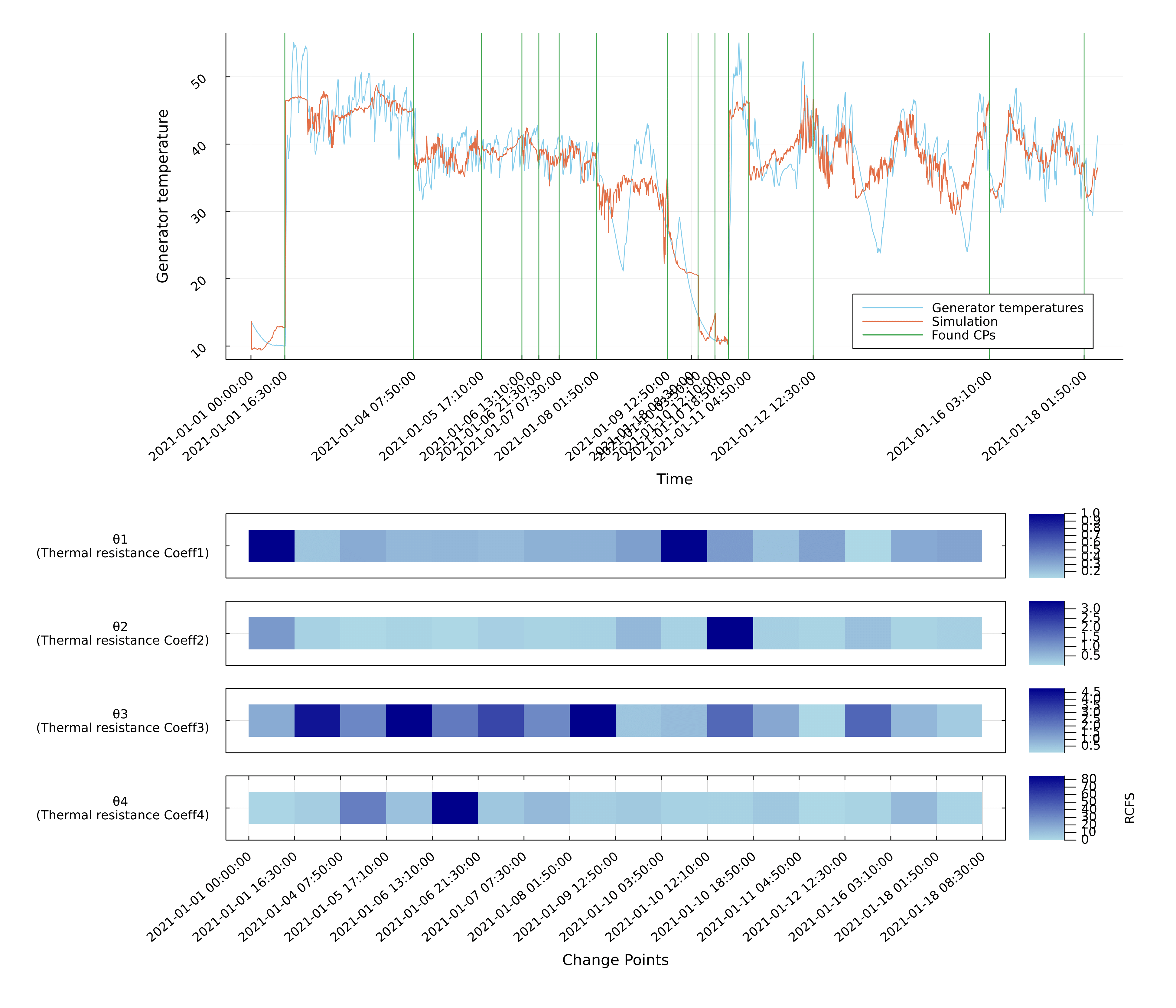
Segment-specific parameters (θ₁–θ₄) represent thermal resistance and cooling dynamics, while non-segment-specific parameters (e.g., copper losses) remain constant across time.
Change Point Detection
Mica detects change points by monitoring structural shifts in the estimated model parameters. The optimization uses a custom objective function based on simulation accuracy, evaluated by comparing model-predicted temperatures with observed SCADA signals.
Each change point marks a period of altered thermal behavior, potentially corresponding to:
- Start-up sequences (e.g., gearbox warm-up, mains run-up)
- External stops due to low wind or icing
- Unreported anomalies in thermal response
Detected change points are automatically aligned with turbine status logs for validation. A detailed alignment table is included in the Supplementary Material.
Results
The figure below shows:
- Top subplot: Observed vs. simulated generator temperature with change points (green lines)
- Bottom subplot: Relative parameter changes (
θ₁–θ₄) across segments, reflecting how cooling efficiency evolves over time.
These parameter shifts provide physical insight into when and how the generator's thermal behavior adapts to operational changes or potential degradation.
We begin by defining the difference equations required for Mica:
Next, we call the changepoint detection function provided by the package to identify both the changepoints and the associated model parameters. The results are shown below:
Example 4: ECG Signal Analysis using ARIMA
Coming soon...